Pop Quiz: Can Linear Regression Optimize Advertising ROI?

Saturday, November 5, 2005

Updated: Saturday, November 4, 2023
The original post has been migrated from a sunset blog host (http://glue.umd.edu/~mmallari/), ported from Minitab to R, Python, and Julia, and refreshed with newer datasets and references.

Soda-Cola, a fictional large-cap beverage company, is facing a rapidly evolving marketplace. Soda-Cola is known for its iconic, refreshing sodas that caters to a loyal customer base. However, the soda market is becoming increasingly competitive as consumers preferences shifted toward healthier options, and new entrants flooded the market with innovative beverages.

To combat this, Soda-Cola is ramping up its advertising efforts across multiple channels: digital platforms (social media and search ads), television, radio, and newspapers. Each channel plays a role in driving brand awareness and sales, but advertising budgets have been allocated based on intuition and historical spending patterns, rather than data-backed decisions.

Leveraging Linear Regression to Optimize Soda-Cola’s Ad Spend

To address this challenge, Soda-Cola’s leadership has greenlit a data-driven initiative to evaluate the impact of advertising spend across all media types on sales. The primary objectives of this project include:

Quantify Channel Effectiveness: Use historical data to identify the relationship between ad spend (digital, TV, radio, and newspaper) and sales.
Optimize Budget Allocation: Determine how to reallocate advertising budgets to maximize sales while minimizing wasted spend.
Develop a Predictive Model: Build a reliable regression model using Linear Regression to forecast sales based on different budget scenarios, enabling proactive rather than reactive decision-making.
Empower the Team with Insights: Equip the marketing team with actionable insights to demonstrate ROI and justify future budget requests.

By applying error-based machine learning (ML)—in this case, linear regression—to uncover the hidden drivers of sales, Soda-Cola aims to transition from guesswork to precision in its marketing strategy. This project would not only provide clarity on past performance but also establish a scalable framework for adapting to future market challenges.

Now that we have context on this marketing problem …

♪ Let’s get technical, technical. I wanna get technical. ♪

Appendix A: Environment, Reproducibility, and Coding Style

If you are interested in reproducing this work, here are the versions of R, Python, and Julia, and the respective packages that I used. Additionally, Leland Wilkinson’s approach to data visualization (Grammar of Graphics) has been adopted for this work. Finally, my coding style here is verbose, in order to trace back where functions/methods and variables are originating from, and make this a learning experience for everyone—including me.

cat(
    R.version$version.string, "-", R.version$nickname,
    "\nOS:", Sys.info()["sysname"], R.version$platform,
    "\nCPU:", benchmarkme::get_cpu()$no_of_cores, "x", benchmarkme::get_cpu()$model_name
)

R version 4.2.3 (2023-03-15) - Shortstop Beagle 
OS: Darwin x86_64-apple-darwin17.0 
CPU: 8 x Intel(R) Core(TM) i5-8259U CPU @ 2.30GHz

require(devtools)
devtools::install_version("dplyr", version="1.1.4", repos="http://cran.us.r-project.org")
devtools::install_version("ggplot2", version="3.5.0", repos="http://cran.us.r-project.org")
devtools::install_version("caret", version="6.0.94", repos="http://cran.us.r-project.org")

library(dplyr)
library(ggplot2)
library(caret)

Python

import sys
print(sys.version)

3.11.4 (v3.11.4:d2340ef257, Jun  6 2023, 19:15:51) [Clang 13.0.0 (clang-1300.0.29.30)]

!pip install pandas==2.0.3
!pip install plotnine==0.12.1
!pip install scikit-learn==1.3.0

import random
import datetime
import pandas
import plotnine
import sklearn

Julia

using InteractiveUtils
InteractiveUtils.versioninfo()

Julia Version 1.9.2
Commit e4ee485e909 (2023-07-05 09:39 UTC)
Platform Info:
  OS: macOS (x86_64-apple-darwin22.4.0)
  CPU: 8 × Intel(R) Core(TM) i5-8259U CPU @ 2.30GHz
  WORD_SIZE: 64
  LIBM: libopenlibm
  LLVM: libLLVM-14.0.6 (ORCJIT, skylake)
  Threads: 1 on 8 virtual cores
Environment:
  DYLD_FALLBACK_LIBRARY_PATH = /Library/Frameworks/R.framework/Resources/lib:/Library/Java/JavaVirtualMachines/jdk1.8.0_241.jdk/Contents/Home/jre/lib/server

using Pkg
Pkg.add(name="HTTP", version="1.10.2")
Pkg.add(name="CSV", version="0.10.13")
Pkg.add(name="DataFrames", version="1.6.1")
Pkg.add(name="CategoricalArrays", version="0.10.8")
Pkg.add(name="StatsBase", version="0.34.2")
Pkg.add(name="Gadfly", version="1.4.0")

using HTTP
using CSV
using DataFrames
using CategoricalArrays
using StatsBase
using Gadfly

Importing and Examining Dataset

Upon importing and examining the dataset, we can see that the data frame dimension is 200 rows and 5 columns.

advertising_r <- read.csv("https://trevorhastie.github.io/ISLR/Advertising.csv")
str(object=advertising_r)

'data.frame':	200 obs. of  5 variables:
 $ X        : int  1 2 3 4 5 6 7 8 9 10 ...
 $ TV       : num  230.1 44.5 17.2 151.5 180.8 ...
 $ radio    : num  37.8 39.3 45.9 41.3 10.8 48.9 32.8 19.6 2.1 2.6 ...
 $ newspaper: num  69.2 45.1 69.3 58.5 58.4 75 23.5 11.6 1 21.2 ...
 $ sales    : num  22.1 10.4 9.3 18.5 12.9 7.2 11.8 13.2 4.8 10.6 ...

head(x=advertising_r, n=8)

  X    TV radio newspaper sales
1 1 230.1    38        69  22.1
2 2  44.5    39        45  10.4
3 3  17.2    46        69   9.3
4 4 151.5    41        58  18.5
5 5 180.8    11        58  12.9
6 6   8.7    49        75   7.2
7 7  57.5    33        24  11.8
8 8 120.2    20        12  13.2

tail(x=advertising_r, n=8)

      X  TV radio newspaper sales
193 193  17   4.1      31.6   5.9
194 194 167  42.0       3.6  19.6
195 195 150  35.6       6.0  17.3
196 196  38   3.7      13.8   7.6
197 197  94   4.9       8.1   9.7
198 198 177   9.3       6.4  12.8
199 199 284  42.0      66.2  25.5
200 200 232   8.6       8.7  13.4

Python

advertising_py = pandas.read_csv("https://trevorhastie.github.io/ISLR/Advertising.csv")
advertising_py.info()

<class 'pandas.core.frame.DataFrame'>
RangeIndex: 200 entries, 0 to 199
Data columns (total 5 columns):
 #   Column      Non-Null Count  Dtype  
---  ------      --------------  -----  
 0   Unnamed: 0  200 non-null    int64  
 1   TV          200 non-null    float64
 2   radio       200 non-null    float64
 3   newspaper   200 non-null    float64
 4   sales       200 non-null    float64
dtypes: float64(4), int64(1)
memory usage: 7.9 KB

advertising_py.head(n=8)

   Unnamed: 0     TV  radio  newspaper  sales
0           1  230.1   37.8       69.2   22.1
1           2   44.5   39.3       45.1   10.4
2           3   17.2   45.9       69.3    9.3
3           4  151.5   41.3       58.5   18.5
4           5  180.8   10.8       58.4   12.9
5           6    8.7   48.9       75.0    7.2
6           7   57.5   32.8       23.5   11.8
7           8  120.2   19.6       11.6   13.2

advertising_py.tail(n=8)

     Unnamed: 0     TV  radio  newspaper  sales
192         193   17.2    4.1       31.6    5.9
193         194  166.8   42.0        3.6   19.6
194         195  149.7   35.6        6.0   17.3
195         196   38.2    3.7       13.8    7.6
196         197   94.2    4.9        8.1    9.7
197         198  177.0    9.3        6.4   12.8
198         199  283.6   42.0       66.2   25.5
199         200  232.1    8.6        8.7   13.4

Julia

advertising_jl = CSV.File(HTTP.get("https://trevorhastie.github.io/ISLR/Advertising.csv").body) |> DataFrames.DataFrame;
describe(advertising_jl)

5×7 DataFrame
 Row │ variable   mean      min   median   max    nmissing  eltype
     │ Symbol     Float64   Real  Float64  Real   Int64     DataType
─────┼───────────────────────────────────────────────────────────────
   1 │ Column1    100.5      1     100.5   200           0  Int64
   2 │ TV         147.043    0.7   149.75  296.4         0  Float64
   3 │ radio       23.264    0.0    22.9    49.6         0  Float64
   4 │ newspaper   30.554    0.3    25.75  114.0         0  Float64
   5 │ sales       14.0225   1.6    12.9    27.0         0  Float64

first(advertising_jl, 8)

8×5 DataFrame
 Row │ Column1  TV       radio    newspaper  sales
     │ Int64    Float64  Float64  Float64    Float64
─────┼───────────────────────────────────────────────
   1 │       1    230.1     37.8       69.2     22.1
   2 │       2     44.5     39.3       45.1     10.4
   3 │       3     17.2     45.9       69.3      9.3
   4 │       4    151.5     41.3       58.5     18.5
   5 │       5    180.8     10.8       58.4     12.9
   6 │       6      8.7     48.9       75.0      7.2
   7 │       7     57.5     32.8       23.5     11.8
   8 │       8    120.2     19.6       11.6     13.2

last(advertising_jl, 8)

8×5 DataFrame
 Row │ Column1  TV       radio    newspaper  sales
     │ Int64    Float64  Float64  Float64    Float64
─────┼───────────────────────────────────────────────
   1 │     193     17.2      4.1       31.6      5.9
   2 │     194    166.8     42.0        3.6     19.6
   3 │     195    149.7     35.6        6.0     17.3
   4 │     196     38.2      3.7       13.8      7.6
   5 │     197     94.2      4.9        8.1      9.7
   6 │     198    177.0      9.3        6.4     12.8
   7 │     199    283.6     42.0       66.2     25.5
   8 │     200    232.1      8.6        8.7     13.4

Wrangling Data

The first column in the dataset represents the index for each row; it’s extraneous and should be dropped. As an option, to start with simple linear regression (SLR), let’s create a new column that combines all the media budget as a single predictor variable. Lastly, let’s clean-up our data frame by reordering the columns (so that the dependent/response variable is the last column) and forcing the column names to be lowercase.

advertising_clean_r <- advertising_r[, -1]
advertising_clean_r$combined_budget <- advertising_r$TV + advertising_r$radio + advertising_r$newspaper
advertising_clean_r <- advertising_clean_r %>% select(-sales, everything(), sales)
colnames(advertising_clean_r) <- tolower(colnames(advertising_clean_r))
str(object=advertising_clean_r)

'data.frame':	200 obs. of  5 variables:
 $ tv             : num  230.1 44.5 17.2 151.5 180.8 ...
 $ radio          : num  37.8 39.3 45.9 41.3 10.8 48.9 32.8 19.6 2.1 2.6 ...
 $ newspaper      : num  69.2 45.1 69.3 58.5 58.4 75 23.5 11.6 1 21.2 ...
 $ combined_budget: num  337 129 132 251 250 ...
 $ sales          : num  22.1 10.4 9.3 18.5 12.9 7.2 11.8 13.2 4.8 10.6 ...

Python

advertising_clean_py = advertising_py.iloc[:, 1:]
advertising_clean_py["combined_budget"] = advertising_clean_py["TV"] + advertising_clean_py["radio"] + advertising_clean_py["newspaper"]
cols = list(advertising_clean_py.columns)
cols.remove('sales')
advertising_clean_py.columns = [col.lower() for col in advertising_clean_py.columns]
advertising_clean_py.info()

<class 'pandas.core.frame.DataFrame'>
RangeIndex: 200 entries, 0 to 199
Data columns (total 5 columns):
 #   Column           Non-Null Count  Dtype  
---  ------           --------------  -----  
 0   tv               200 non-null    float64
 1   radio            200 non-null    float64
 2   newspaper        200 non-null    float64
 3   sales            200 non-null    float64
 4   combined_budget  200 non-null    float64
dtypes: float64(5)
memory usage: 7.9 KB

Julia

advertising_clean_jl = advertising_jl[:, Not(1)];
advertising_clean_jl.combined_budget = advertising_clean_jl.TV + advertising_clean_jl.radio + advertising_clean_jl.newspaper;
advertising_clean_jl = select(advertising_clean_jl, Not(:sales), :sales);
rename!(advertising_clean_jl, lowercase.(names(advertising_clean_jl)));
describe(advertising_clean_jl)

5×7 DataFrame
 Row │ variable         mean      min      median   max      nmissing  eltype
     │ Symbol           Float64   Float64  Float64  Float64  Int64     DataType
─────┼──────────────────────────────────────────────────────────────────────────
   1 │ tv               147.043       0.7   149.75    296.4         0  Float64
   2 │ radio             23.264       0.0    22.9      49.6         0  Float64
   3 │ newspaper         30.554       0.3    25.75    114.0         0  Float64
   4 │ combined_budget  200.861      11.7   207.35    433.6         0  Float64
   5 │ sales             14.0225      1.6    12.9      27.0         0  Float64

first(advertising_clean_jl, 8)

8×5 DataFrame
 Row │ tv       radio    newspaper  combined_budget  sales
     │ Float64  Float64  Float64    Float64          Float64
─────┼───────────────────────────────────────────────────────
   1 │   230.1     37.8       69.2            337.1     22.1
   2 │    44.5     39.3       45.1            128.9     10.4
   3 │    17.2     45.9       69.3            132.4      9.3
   4 │   151.5     41.3       58.5            251.3     18.5
   5 │   180.8     10.8       58.4            250.0     12.9
   6 │     8.7     48.9       75.0            132.6      7.2
   7 │    57.5     32.8       23.5            113.8     11.8
   8 │   120.2     19.6       11.6            151.4     13.2

last(advertising_clean_jl, 8)

8×5 DataFrame
 Row │ tv       radio    newspaper  combined_budget  sales
     │ Float64  Float64  Float64    Float64          Float64
─────┼───────────────────────────────────────────────────────
   1 │    17.2      4.1       31.6             52.9      5.9
   2 │   166.8     42.0        3.6            212.4     19.6
   3 │   149.7     35.6        6.0            191.3     17.3
   4 │    38.2      3.7       13.8             55.7      7.6
   5 │    94.2      4.9        8.1            107.2      9.7
   6 │   177.0      9.3        6.4            192.7     12.8
   7 │   283.6     42.0       66.2            391.8     25.5
   8 │   232.1      8.6        8.7            249.4     13.4

Performing Exploratory Data Analysis (EDA)

Univariate Analysis

ggplot2::ggplot(advertising_clean_r, aes(x=sales)) +
    geom_histogram()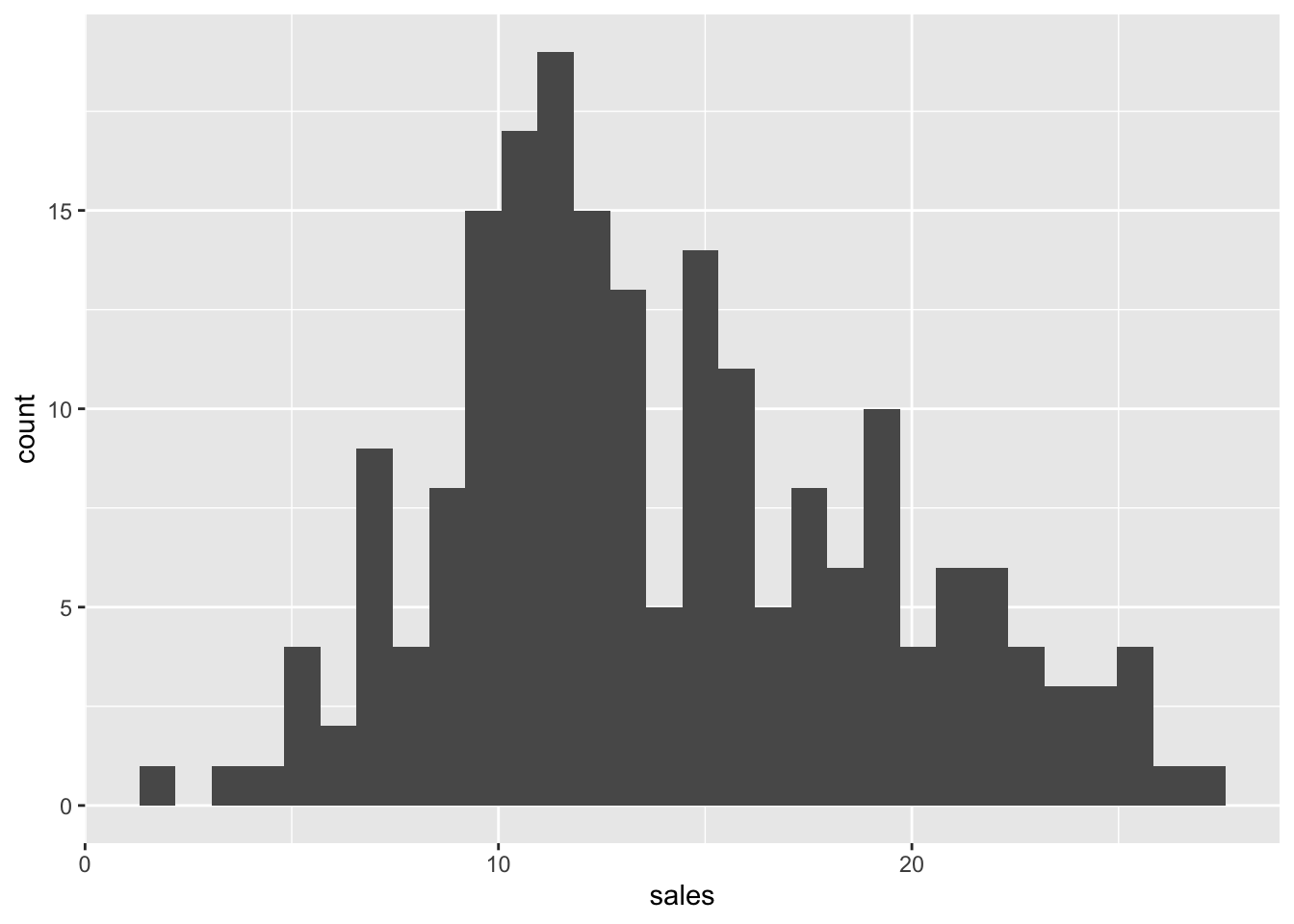

summary(advertising_clean_r$sales)

   Min. 1st Qu.  Median    Mean 3rd Qu.    Max. 
    1.6    10.4    12.9    14.0    17.4    27.0

Python

advertising_clean_py.describe()

               tv       radio   newspaper       sales  combined_budget
count  200.000000  200.000000  200.000000  200.000000       200.000000
mean   147.042500   23.264000   30.554000   14.022500       200.860500
std     85.854236   14.846809   21.778621    5.217457        92.985181
min      0.700000    0.000000    0.300000    1.600000        11.700000
25%     74.375000    9.975000   12.750000   10.375000       123.550000
50%    149.750000   22.900000   25.750000   12.900000       207.350000
75%    218.825000   36.525000   45.100000   17.400000       281.125000
max    296.400000   49.600000  114.000000   27.000000       433.600000

Julia

describe(advertising_clean_jl.sales)

Summary Stats:
Length:         200
Missing Count:  0
Mean:           14.022500
Minimum:        1.600000
1st Quartile:   10.375000
Median:         12.900000
3rd Quartile:   17.400000
Maximum:        27.000000
Type:           Float64

Bivariate Analysis

ggplot2::ggplot(advertising_clean_r, aes(x=combined_budget, y=sales)) +
    geom_point()

cor(x=advertising_clean_r$combined_budget, y=advertising_clean_r$sales, method="pearson")

[1] 0.87

ggplot2::ggplot(advertising_clean_r, aes(x=combined_budget, y=tv)) +
    geom_point()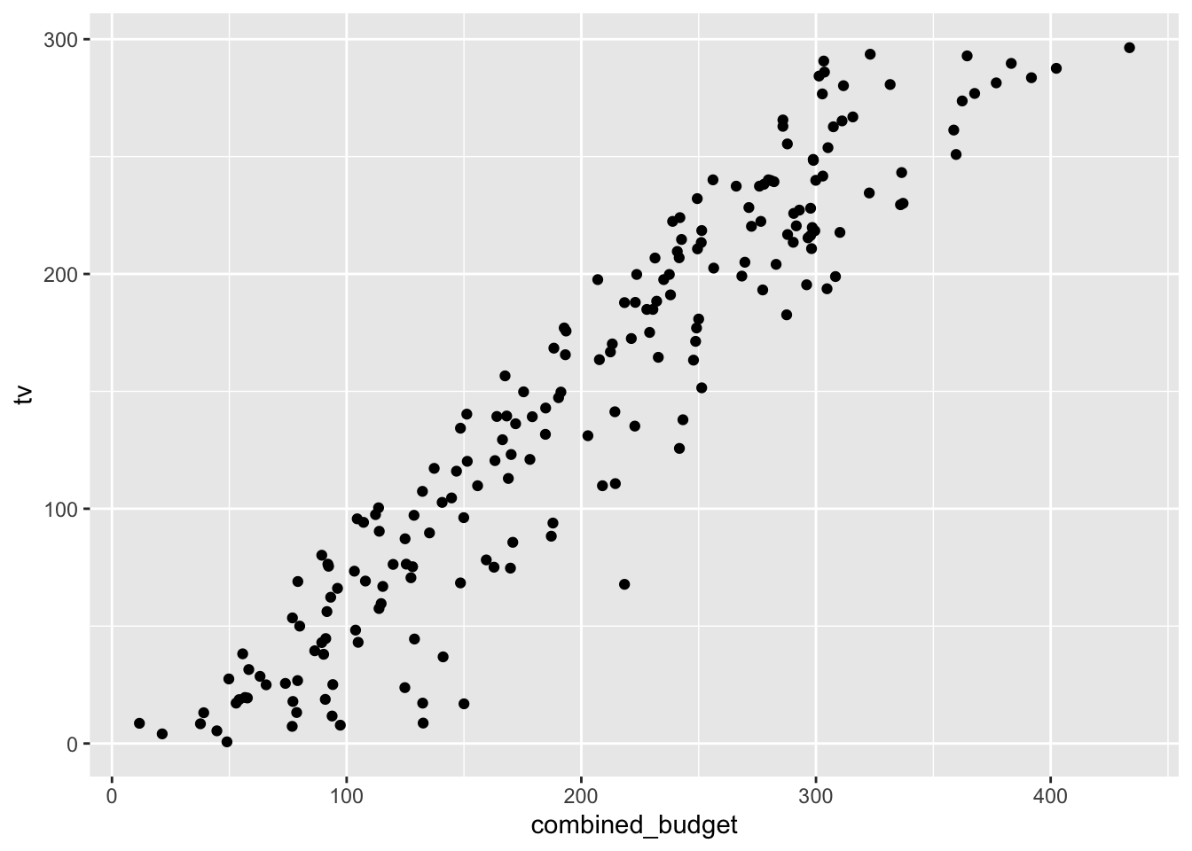

cor(x=advertising_clean_r$tv, y=advertising_clean_r$sales, method="pearson")

[1] 0.78

ggplot2::ggplot(advertising_clean_r, aes(x=radio, y=sales)) +
    geom_point()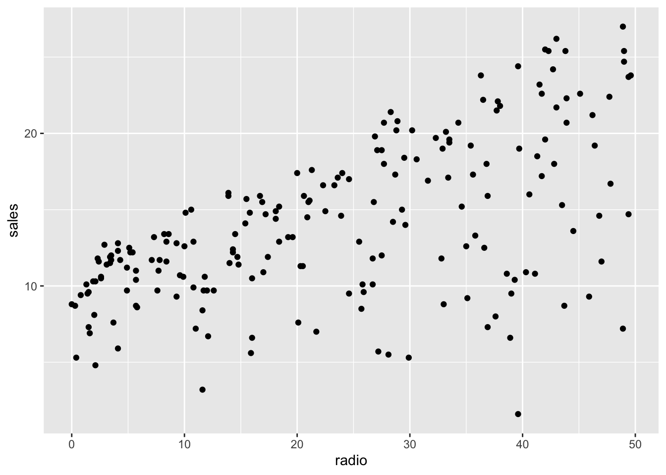

cor(x=advertising_clean_r$radio, y=advertising_clean_r$sales, method="pearson")

[1] 0.58

ggplot2::ggplot(advertising_clean_r, aes(x=newspaper, y=sales)) +
    geom_point()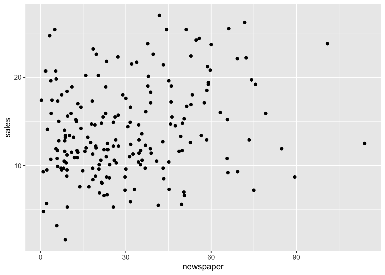

cor(x=advertising_clean_r$newspaper, y=advertising_clean_r$sales, method="pearson")

[1] 0.23

Python

Julia

Splitting Data for Training & Testing

set.seed(1856)
index_train <- createDataPartition(advertising_clean_r$sales, p=0.7, list=FALSE, times=1)
advertising_clean_train_r <- advertising_clean_r[index_train, ]
advertising_clean_test_r <- advertising_clean_r[-index_train, ]
dim(advertising_clean_train_r)

[1] 142   5

dim(advertising_clean_test_r)

[1] 58  5

Python

Julia

# walmart_clean_stratified_train_julia,
# walmart_clean_stratified_test_julia = MLJ.partition(
#     walmart_clean_jl,
#     0.7,
#     rng = 1856,
#     stratify = walmart_clean_jl.store
# );
# size(walmart_clean_stratified_train_julia)

# histogram_store_train_julia = Gadfly.plot(
#     walmart_clean_stratified_train_julia,
#     x = "store",
#     Gadfly.Geom.histogram(maxbincount = 45),
#     Gadfly.Guide.xlabel("Store ID"),
#     Gadfly.Guide.ylabel("Count"),
#     michaelmallari_theme
# );

# size(walmart_clean_stratified_test_julia)
# histogram_store_test_julia = Gadfly.plot(
#     walmart_clean_stratified_test_julia,
#     x = "store",
#     Gadfly.Geom.histogram(maxbincount = 45),
#     Gadfly.Guide.xlabel("Store ID"),
#     Gadfly.Guide.ylabel("Count"),
#     michaelmallari_theme
# );

Fitting For Linear Model (Simple Linear Regression)

slr_fit_r <- lm(
    formula=sales ~ combined_budget,
    data=advertising_clean_train_r
)
summary(slr_fit_r)


Call:
lm(formula = sales ~ combined_budget, data = advertising_clean_train_r)

Residuals:
   Min     1Q Median     3Q    Max 
-7.165 -1.444  0.073  1.691  7.213 

Coefficients:
                Estimate Std. Error t value             Pr(>|t|)    
(Intercept)      4.14858    0.50920    8.15     0.00000000000019 ***
combined_budget  0.04895    0.00228   21.48 < 0.0000000000000002 ***
---
Signif. codes:  0 '***' 0.001 '**' 0.01 '*' 0.05 '.' 0.1 ' ' 1

Residual standard error: 2.5 on 140 degrees of freedom
Multiple R-squared:  0.767,	Adjusted R-squared:  0.766 
F-statistic:  462 on 1 and 140 DF,  p-value: <0.0000000000000002

Python

Julia

slr_fit_julia = lm(
    @formula(sales ~ combined_budget,
    advertising_clean_julia
)

Fitting For Linear Model (Multiple Linear Regression)

mlr_fit_r <- lm(
    formula=sales ~ tv + radio + newspaper,
    data=advertising_clean_train_r
)
summary(mlr_fit_r)


Call:
lm(formula = sales ~ tv + radio + newspaper, data = advertising_clean_train_r)

Residuals:
   Min     1Q Median     3Q    Max 
-5.101 -0.935  0.200  1.160  2.823 

Coefficients:
            Estimate Std. Error t value             Pr(>|t|)    
(Intercept)  2.97682    0.35515    8.38    0.000000000000054 ***
tv           0.04600    0.00153   30.02 < 0.0000000000000002 ***
radio        0.18931    0.00982   19.28 < 0.0000000000000002 ***
newspaper   -0.00445    0.00639   -0.70                 0.49    
---
Signif. codes:  0 '***' 0.001 '**' 0.01 '*' 0.05 '.' 0.1 ' ' 1

Residual standard error: 1.6 on 138 degrees of freedom
Multiple R-squared:  0.909,	Adjusted R-squared:  0.908 
F-statistic:  462 on 3 and 138 DF,  p-value: <0.0000000000000002

Python

Julia

Pop Quiz: Can Linear Regression Optimize Advertising ROI?

Uncovering Budget Blind Spots From Ineffective Advertising Allocation

Leveraging Linear Regression to Optimize Soda-Cola’s Ad Spend

Appendix A: Environment, Reproducibility, and Coding Style

Importing and Examining Dataset

Wrangling Data

Performing Exploratory Data Analysis (EDA)

Univariate Analysis

Bivariate Analysis

Splitting Data for Training & Testing

Fitting For Linear Model (Simple Linear Regression)

Fitting For Linear Model (Multiple Linear Regression)

Making Predictions With Test Data

Evaluating Model Predictions

Further Readings